1
2
3

import numpy as np
import matplotlib.pyplot as plt
%matplotlib inline

描述控制系统

在这一部分,假设$u(t)$为系统某一时刻的输入,$y(t)$为系统某一时刻的输出$t$为时间

利用递推法即$y_n=\Sigma f(y_k)+g(u_n)$,我们可以得到一个齐次线性微分方程描述输出和输入之间的关系
$$\Sigma_k^n\frac{\mathbb{d}^k}{\mathbb{d}t^k}a_ky(t)=\Sigma_i^n\frac{\mathbb{d}^i}{\mathbb{d}t^i}b_ku(t)$$

对于一些特殊情况,例如系统的状态与其历史无关,那么系统可以被简化为$y(t)=b_0u(t)$
下面将对一个常见模型进行建模

Fitting points

We chose three typical points from the HID graph.

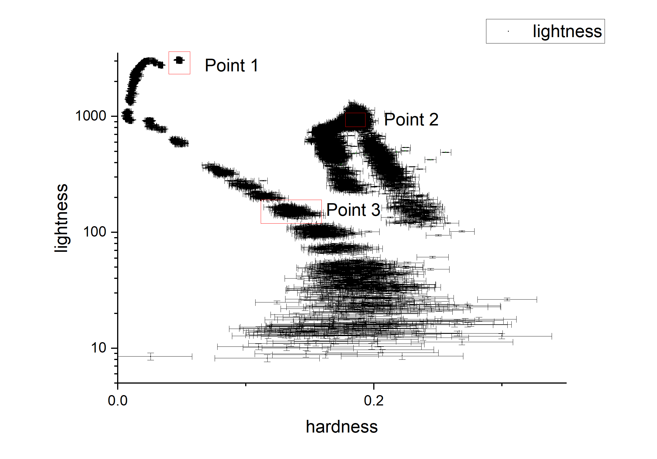
The first point

The first point is the observation is the three observation in P14661084 and we use the low energy and mid energy part of the spectrum.

We combine the spectra in P14661084 and use the model constant*TBabs*(simplcutx*(diskbb+relxillCp)+xillverCp)(The reason why I didn’t use the model mbknpo is that if I add this model, then the spectrum of the very low energy(about 2keV) may not fit well), and I got the best-fit like this.

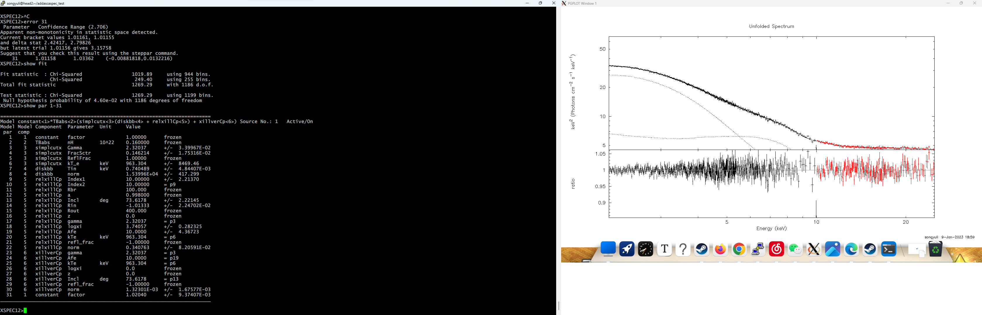
Also, we calculate the error of each parameter, and got the table below

The second point

The second point is the three observation in ``, we used all the energy part of the spectrum.

Also, we used the model constant*TBabs*(simplcutx*(diskbb+relxillCp)+xillverCp)to fit the spectrum. And ignored the spectrum between 21keV to 23keV. This time, however, we found that the model cannot fit the spectrum very well, especially at about Fe-line and at about 25 keV.

The unfolded spectrum and the ratio is like below:

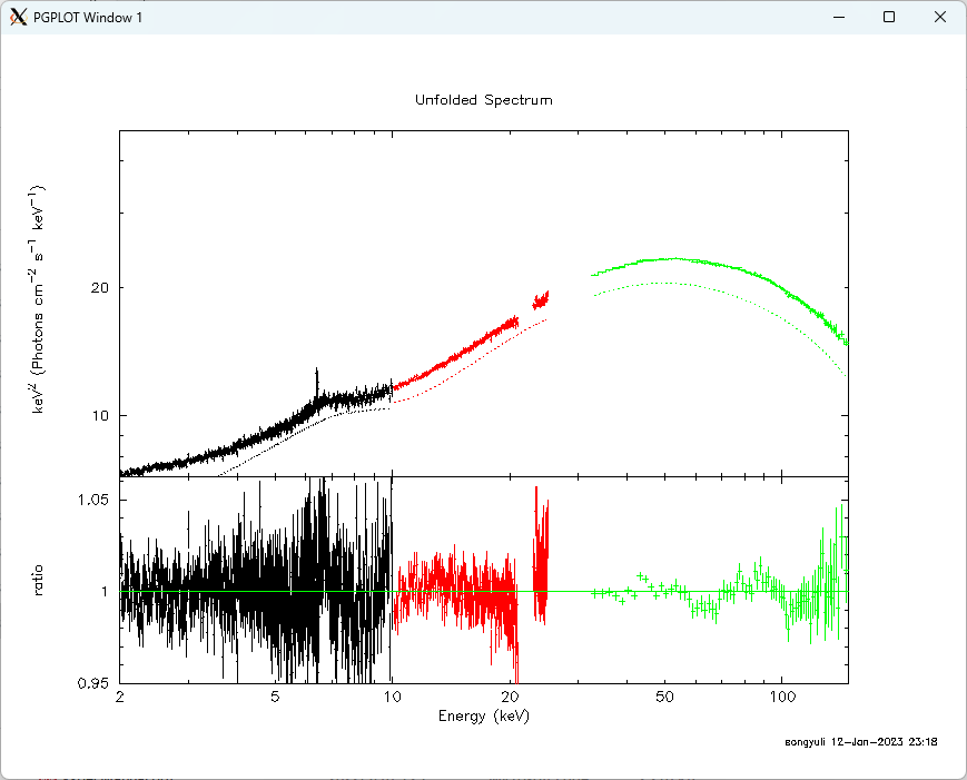
We calculated the error of each parameter, and got the table below:

I noticed that the range of the parameter Rin is quite large, which may be related to the unfitted Fe-line.

The third point

The second point is the two observation in P0114661136, we used all the energy part of the spectrum.

We use the model constant*TBabs*(simplcutx*(diskbb+mbnkpo*relxillCp)+xillverCp) to fit the spectrum. And ignored the spectrum between 21keV to 23keV. This time except the problem at about 20keV and 25keV, the model can fit the spectrum quite well.

The unfolded spectrum and the ratio is like below: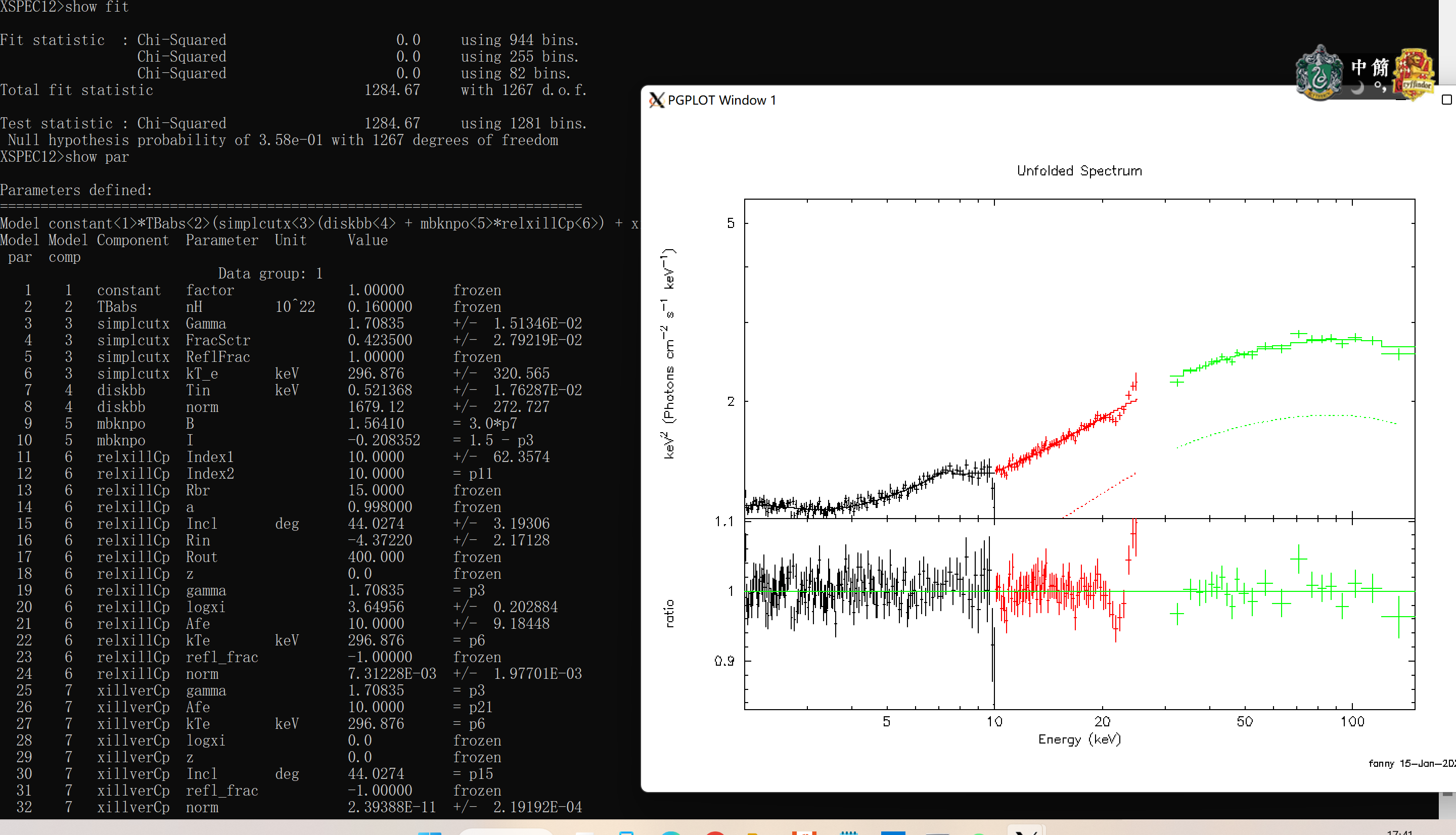

We calculated the error of each parameter, and got the table below:

Discussions

1. In real world ,the Incl should not change with time, so we should fix it to some value (In the ==NuSTAR== it is 63, but we’ve found that it cannot fit very well)
2. We don’t need to get the best fit because our goal is to fit all the observations, so if the Reduced Chi-Squared(Chi-Squared/Degrees of freedom)is under 1.2,although it is still not the best fit ,it would be ok.

被控对象的行为

准备工作

为了更加方便地绘制相关图像,在这里要进行相应的准备工作

1
2
3
4

import matplotlib.pyplot as plt
import numpy as np
import control as ct 
from control.matlab import *

绘图时用以确定线条类型

1
2
3
4
5
6

def line_generator():
    linestyle=["-","--","-.",":"]
    lineid=0
    while True:
        yield linestyle[lineid] #* 这个yield用法很有趣,可以学习一下
        lineid=(lineid+1)%len(linestyle)

用以完善绘图

1
2
3
4
5
6

def plot_set(fig_ax,*args):
    fig_ax.set_xlabel(args[0])
    fig_ax.set_ylabel(args[1])
    fig_ax.grid(ls=':')
    if len(args)==3:
        fig_ax.legend(loc=args[2])

用以完善伯德图函数

1
2
3
4
5
6
7
8
9
10

def bodeplot_set(fig_ax,*args):
    fig_ax[0].grid(which='both',ls=':')
    fig_ax[0].set_ylabel('Gain [dB]')
    fig_ax[1].grid(which='both',ls=':')
    fig_ax[1].set_xlabel('$\omega$ [rad/s]')
    fig_ax[1].set_ylabel('Phase [deg]')
    if len(args)>0:
        fig_ax[1].legend(loc=args[0])
    if len(args)>1:
        fig_ax[0].legend(loc=args[1])

时域响应

This is the introduction and index of my blog, and it’s for testing the Hexo.

My plans and projects

This is the list of my plans and projects.

Some of them would be written in Chinese and some of them would be written in English(awful English).

• A magnetic field sensor based on a 3D printer(3D 位移平台)

• Study the spectrum of maxi1820(maxi1820)

• Make and improve a python library to process the uncertainty

• Some other useful tools

My study plans

Also, I need to learn some interesting thing, the list can be the index of my notes

• Controlling system with python(Python设计控制系统)

• Machine learning(机器学习)

• Analyzing X-ray spectrum from BH(X-ray spectrum)

• Statics(统计学)

My logs

Sometimes there are interesting logs in my project and study, most of them may be about Python and Linux.